Self-Referential Structures on Dependency Graphs

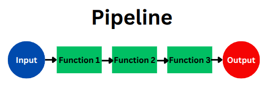
In previous chapters, we’ve explored the powerful concept of the data transformation pipeline, where data sequentially passes through a series of functions. This illustrates a clear flow of data from input to output.

Pipeline image

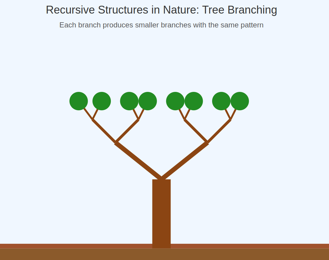
On the other hand, in the chapter “Recursion: The Foundation of Functional Iteration,” we delved into the fundamentals of loops in functional programming, where functions achieve repetition by calling themselves. As explained in that chapter, self-reference itself suggests loop structures or circular dependencies.

escher-img Hand with Reflecting Sphere, also known as Self-Portrait in Spherical Mirror by M. C. Escher

tree-img

A question might arise here: How does the concept of a one-way pipeline relate to structures that refer to themselves and loop? In particular, “loops” created by self-reference or recursive definitions don’t seem to fit directly into a simple linear pipeline model.

The key to answering this question lies in the Dependency Graph.

Representing Self-Referential Structures with Dependency Graphs

Now, using this concept of a dependency graph, how are “self-reference” and “recursion,” which we discussed in the previous chapter, represented?

When depicting self-referential structures in a dependency graph, the representation method varies slightly depending on whether the reference is direct or indirect, and what the nodes of the graph represent. However, it fundamentally appears as a “cycle” or “self-loop” within the graph.

Let’s explain with a few patterns:

Direct Self-Reference
- This occurs when an element (node) directly refers to or depends on itself.
- Representation in a dependency graph: It’s drawn as a self-loop edge, originating from and returning to the same node.
```
 A
 ↻
```
  (Node A depends on itself)
- Examples:
  - Recursive function: If a function f calls itself internally (like the sumUpTo function from the previous chapter), a self-loop is formed on the node representing f.
  - Data structure: When an object has a pointer or reference to an instance of itself.
  - State transition: When a state S, under certain conditions, transitions back to state S.
Indirect Self-Reference / Circular Dependency
- This occurs when an element A depends on another element B, which in turn depends on another element C, and eventually, C depends back on A.
- Representation in a dependency graph: It’s drawn as a cycle, where a path of multiple nodes and edges leads back to the starting node.
```
A ━━━▶ B
▲       │
│       ▼
D ◀━━━ C
```
  (In this example, there’s a cycle A → B → C → D → A, meaning A, B, C, and D are indirectly self-referential.)
- Examples:
  - Mutually recursive functions: Function f calls function g, and function g calls function f (f <-> g).
  - Circular dependencies between modules: Module A uses functionality from Module B, and Module B uses functionality from Module A.
  - Circular references in object-oriented programming: Object A holds a reference to Object B, and Object B also holds a reference to Object A.

Implications and Caveats of Self-Reference (Cycles) in Dependency Graphs

In the previous chapter, “Recursion: The Foundation of Functional Iteration,” under “The Concept of Self-Reference,” we encountered the following insight:

Viewing recursion through the lens of self-reference allows us to understand it as a more universal, even philosophical concept that transcends mere programming techniques. The act of referring to oneself holds both infinite possibilities and potential contradictions, which contributes to the depth and fascination of recursion.

This phrase, “infinite possibilities and potential contradictions,” offers a crucial insight for understanding the meaning of cycles when self-reference appears as a “cycle” or “self-loop” in a dependency graph.

A cycle in a dependency graph can be seen as a mirror reflecting this duality:

One aspect of “infinite possibilities” manifests as the power to solve complex problems or represent efficient data structures by repeatedly executing computations as intended. Examples include iterative processes in convergence calculations or the representation of data structures like circular lists.
On the other hand, one aspect of “potential contradictions” manifests as problems like “infinite loops,” where computation never ends unless controlled, or “deadlocks,” where processes wait for each other’s completion and no progress is made.

Therefore, when a cycle is found in a dependency graph, it’s necessary to carefully interpret which aspect it reflects.

Here’s a breakdown of specific caveats and implications:

Computability/Executability (The “Potential Contradictions” Aspect):
- If a cycle exists in a dependency graph that shows the order of task execution (like a workflow), it often suggests the possibility of a “deadlock” or an “infinite loop.” This means a situation like A can’t finish until B starts, and B can’t start until A finishes. This is structurally the same as the problem discussed in the previous chapter where a recursive function without a base case falls into infinite calls, leading to a stack overflow.
- In such cases, the dependency graph is usually expected to be a Directed Acyclic Graph (DAG). If it’s a DAG, the start and end points of processing are clear, and infinite loops don’t occur.
Representing Data Structures (The “Infinite Possibilities” Aspect):
- In graphs representing reference relationships in data structures, structures intentionally designed with cycles exist, such as circular lists or groups of mutually referencing objects. This isn’t an error but a representation of the inherent characteristics of that data structure, an example harnessing the “possibilities” of self-reference.
Iterative Computations/Convergence (The “Infinite Possibilities” Controlled Aspect):
- Some scientific computations and algorithms involve repeating a calculation until a value meets a specific condition (e.g., converges). This is conceptually a self-referential structure—“the result of the current step becomes the input for the next step”—and is represented as a self-loop or cycle in a dependency graph.
- This type of cycle, like a recursive function with Tail Call Optimization (TCO) or a recursion with a proper base case (as seen in the previous chapter), is a “controlled” repetition and an effective means for problem-solving. Here too, the “possibilities” of self-reference are constructively utilized.
Granularity of the Graph:
- How self-reference is depicted also depends on the level of detail (granularity) at which the graph’s nodes are defined. For instance, if an entire recursive function is a single node, it becomes a self-loop. Conversely, if each recursive call is (theoretically) expanded as an individual node, it might look like a deep tree structure (though its tips would head towards base cases).

The Decisive Difference Between Iterative/Convergent Computations and Infinite Loops: The Key to Avoiding “Potential Contradictions” and Harnessing “Possibilities”

Among things represented as cycles in a dependency graph, there are two types: intended iterative/convergent computations that leverage constructive “infinite possibilities,” and uncontrolled infinite loops which are program errors where “potential contradictions” become manifest. Though they might look similar, their natures are fundamentally different.

The most crucial factor distinguishing these two—and the key to avoiding “potential contradictions” while constructively harnessing “possibilities”—is the presence (and appropriateness) of “termination conditions” and a “path to exit the loop.”

Iterative/Convergent Computations (Controlled Cycles):
- Purpose: To iteratively improve an approximate solution until it reaches a certain precision (converges), or to perform a calculation a predetermined number of times to obtain a final result.
- Termination Conditions (Path to Exit Loop):
  - Convergence Check: When the difference between the result of the previous step and the current step falls below a preset tolerance (e.g., epsilon).
  - Maximum Iteration Count: When the number of computations reaches an upper limit (to prevent divergence if convergence isn’t achieved).
  - Achievement of a Specific State: When specific conditions related to the problem’s nature are met. (This is similar to the role of a base case in recursion.)
- When these termination conditions are met, the iterative process stops, and the obtained result is used to proceed to the next process, or the computation is completed. That is, a path to exit the cycle is clearly defined.
- Representation in a Dependency Graph: Even if drawn as a cycle, the logic controlling the cycle (checking termination conditions) is understood to exist, either implicitly as part of the node’s internal logic or explicitly as control nodes or conditional branch edges in the graph.
(Problematic) Infinite Loops (Uncontrolled Cycles):
- Cause (Lack of Purposeful Design): Often due to design flaws or bugs, termination conditions are unintentionally not met, or no termination condition exists in the first place.
- Termination Conditions: Effectively non-existent or set to logically unreachable conditions.
- Exit from Loop: Cannot exit the loop without external forced intervention.
- Representation in a Dependency Graph: Depicted as a cycle, indicating a state where there’s no effective path or control mechanism to exit the cycle. This causes deadlocks or system hangs.

Addendum on Representing Termination Conditions in Dependency Graphs:

In a simple dependency graph, a self-loop like A --> A might be drawn to show that node A is executed iteratively. The termination condition isn’t explicit in this diagram itself. It’s often interpreted as being implemented within A’s “internal logic” or by an external mechanism managing its execution.
In more detailed representations, like a Control Flow Graph, the entry and exit points of an iteration block, as well as conditional branching (to continue or exit the loop), are explicitly drawn. In this case, the “path to exit the loop” is represented as a clear edge on the graph.

Cycles in iterative or convergent computations are thus “controlled repetitions” with clear exit strategies. It’s crucial to understand that this is fundamentally different from an infinite loop where processing simply never ends, especially when interpreting these in the context of dependency graphs.

In Summary

A self-referential structure is depicted in a dependency graph as a self-loop (for direct self-reference) emerging from and returning to the same node, or as a cycle (for indirect self-reference) where multiple nodes and edges lead back to an origin node.

As touched upon in the previous chapter, self-reference encapsulates “infinite possibilities and potential contradictions.” Similarly, cycles in a dependency graph require careful interpretation.

In graphs showing task execution order, a cycle often suggests a manifestation of “potential contradictions,” indicating problems like infinite loops or deadlocks. Thus, a Directed Acyclic Graph (DAG) is generally preferred.
However, when modeling recursive algorithms or iterative computations, a cycle is an intentional and indispensable structure embodying “infinite possibilities.” For such repetitions to be computable (i.e., to eventually terminate), the presence and appropriateness of “termination conditions” and a “path to reach them” are critically important. This is the dividing line between constructive iterative processes and problematic, uncontrolled infinite loops.

Dependency graphs thus provide a powerful framework for uniformly representing diverse computational patterns—from simple linear processes to complex patterns woven by self-reference—along with both the “possibilities” and “contradictions” they entail.